Hopfield Neural Network
Implementation & Demo
https://github.com/slynj/hopfield-neural-network
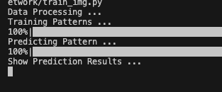
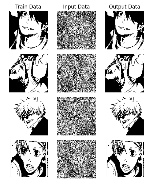
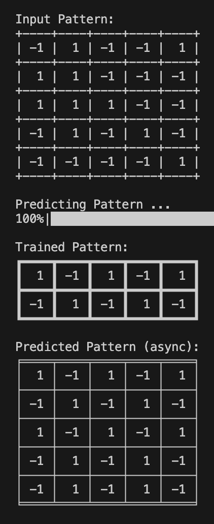
Demo with Corrupted Images
Run train_img.py
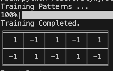
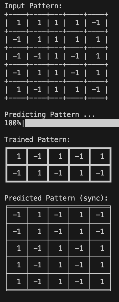
Demo with Simple Matrix
Run train_test.py
| Training | Sync | Async |
|---|---|---|
 |
 |
 |
Introduction
- Invented by Dr John J. Hopfied, consists of 1 layer of \(N\) fully connected recurrent neurons.
- Type of recurrent neural network (RNN).
- One of the earliest conceptualization of biological neural networks.
- Designed to remember patterns and retrieve them when given incomplete/noisy data.
- Brain inspired memory system ⇒ can recall complete memories from partial hints (like how you can recognize a blurry face of a friend and read horrible handwritings)
- Generally used in associative memory/optimization tasks.
Discrete Hopfield Network
- Fully connected neurons → every neuron is connected to every other neurons
- Neuron states → Bipolar (-1, 1)
- Symmetric Weights → \(w_{ij} = w_{ji}\) , no self-connections ( \(w_{ii} = 0\) )
- the connection weight between 2 neurons is the same in both directions (\(w_{ij} = w_{ji}\)).
- Also, weight to itself is 0 (\(w_{ii}=0\)). (\(w_{ij}\) is weight associated with the connection between the \(i\)th and the \(j\)th neuron)
- Each neuron has an inverting and a non-inverting output.
- inverting: passes on the oppposite state as it receives (1 ⇒ -1, -1 ⇒ 1)
- non-inverting: passes on the same state as it receives
- Associative (Hebbian) learning
- Neurons update themselves based on other neuron’s output
Structure & Architecture
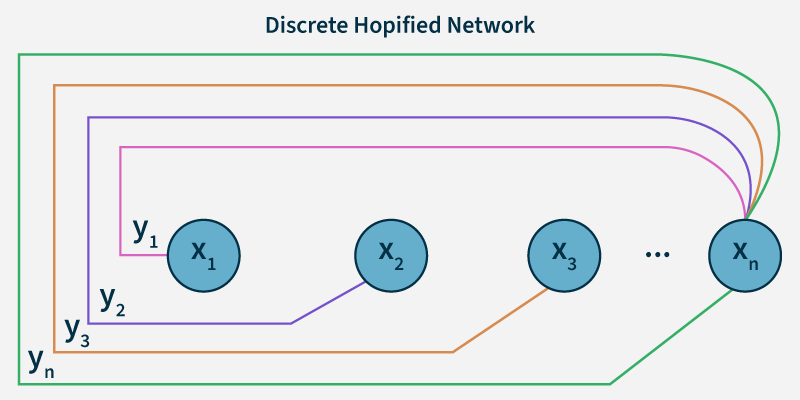
- \(x_1, x_2, \cdots, x_n\): input to \(n\) given neurons
- \(y_1, y_2, \cdots, y_n\): outputs from \(n\) given neurons
- Since they’re fully connected, output of each neurons (\(y_1,y_2, \cdots y_n\)) are inputs to the rest of the neurons excluding itself.
Energy Function
- Hopfield network is an energy based model.
- When the network receives the corrupted pattern, it updates the neurons iteratively to minimize the energy ⇒ at the end converge to the closest stored pattern.
- The network’s goal is to minimize the value of the energy function ⇒ where the energy minimizes is what the saved pattern is (associated memory).
- So even if the input is disrupted or not complete, it tries to reach the pattern ⇒ converges to the local minima.
- \(E = -\frac{1}{2} \sum_{i \neq j} w_{ij} s_i s_j + \sum_i \theta_i s_i\)
- \(s_i\) : neuron \(i\)’s current state (-1/1 or 0/1)
- \(w_{ij}\) : neuron \(i\) and \(j\)’s weight (symm.)
- \(\theta\) : threshold of neuron \(i\) (determines whether the neuron will be activated (1) or deactivated (-1) based on the total input it receives from other neurons.)
Hebbian Learning
- Learning rule used to store the pattern ⇒ calculate the weights.
- Core idea: If 2 neurons activate simultaneously, their synaptic connection strengthens (ie. heavier weight).
- \(w_{ij} = \frac{1}{N} \sum_{\mu=1}^{P} \xi_i^{\mu} \xi_j^{\mu}\)
- \(N\) : # of neurons
- \(P\) : # of patterns to store
- \(\xi_i^{\mu}\) : neuron \(i\)’s state on the \(\mu\)th pattern
- \(ξ\) : state / state pattern
-
“Neurons that fire together wire together”
-
If \(\xi_i^{\mu} = 1\) and \(\xi_j^{\mu} = 1\), \(\xi_i^{\mu} \xi_j^{\mu} = 1\)
-
If one of them is -1, \(\xi_i^{\mu} \xi_j^{\mu} = -1\)
- ⇒ when they’re in the same states together, the corresponding weight increases (vice versa).
-
Simple, and can store multiple patterns.
- However overlapping patterns can cause errors and it does not forget or adapt new info.
Training Algorithm
- Initialize the network
- determine the # of stored patterns
- get the # of neurons in each pattern
- init the weight matrix
- Compute the Average Neuron Activation(rho; \(\rho\) )
- \(\rho\) : avg activation value of all neurons across all patterns
- sum of all vals / num of vals
- helps prevent one pattern from dominating the network
- ex. network could overfit if there’s a pattern with all 1s. (\(\rho\) prevents it)
- subtracting rho makes learning stable by prevent the network from biasing on a particular pattern. (state - rho → then used for dot product for weight calculation)
- \(\rho\) : avg activation value of all neurons across all patterns
- Hebbian Learning
- for each patern in the dataset,
- subtract rho from the pattern to center the values
- computer the outer product and add it to the weight matrix
- for each patern in the dataset,
- Normalize Values
- divide the weight matrix by the number of data (not the # of vals) → prevents the weights from getting large